Introduction to the crunchflow.output package
The crunchflow.output package is designed to support analyses with the reactive transport code CrunchFlow. It provides classes for analyzing spatial and time series output from CrunchFlow simulations.
1. Loading and Plotting TimeSeries Data
The TimeSeries class is designed to work with time series data output from CrunchFlow simulations using the time_series_print key. The output contains time-varying concentrations at an individual grid cell. Here’s an example:
[1]:
# Import the TimeSeries class
from crunchflow.output import TimeSeries

# Load a sample time series file as a TimeSeries object
# We simply provide the name and location of the file
ts = TimeSeries("ObservationWell01.txt", folder="output_files")

# Now that we've loaded it in, this TimeSeries object has methods
# and attributes associated with it. For example, we can print the
# coordinate (grid cell) at which this time series was recorded
print("(x, y, z):", ts.coords)
(x, y, z): (100, 1, 1)
[2]:
# We can also print a list of the species included in this file
print("Species:", ts.species)
Species: ['pH', 'H+', 'CO3--', 'SO4--', 'Cl-', 'Ca++', 'Mg++', 'Na+', 'K+', 'Fe++', 'Fe+++', 'HS-', 'CH3COO-', 'O2(aq)', 'S(aq)', 'Br-', 'CH3COOH(aq)', 'CaOH+', 'CaCH3COO+', 'CaHCO3+', 'CaCO3(aq)', 'CaSO4(aq)', 'H2CO3(aq)', 'HCO3-', 'FeOH+', 'FeCH3COO+', 'FeHCO3+', 'FeCO3(aq)', 'Fe(CO3)2--', 'FeSO4(aq)', 'FeCl+', 'Fe(HS)2(aq)', 'Fe(HS)3-', 'H2S(aq)', 'S--', 'KSO4-', 'MgOH+', 'MgCH3COO+', 'MgHCO3+', 'MgCO3(aq)', 'MgSO4(aq)', 'NaCH3COO(aq)', 'NaHCO3(aq)', 'NaCO3-', 'NaSO4-', 'HSO4-', 'OH-']
[3]:
# These are a couple of the attributes associated with the object. To
# get a list of all of the object's attributes, we can use the `__dict__`
# method, which prints a dictionary of all the object's attributes and their
# values. Note that we're only printing out the keys (the attribute names)
# of the dictionary, since the values can be quite long.
print("Current attributes:", ts.__dict__.keys())
Current attributes: dict_keys(['coords', 'columns', 'species', 'timeunit', 'unit', 'data', 'df'])
[4]:
# From the keys above, we can see that another TimeSeries object attribute
# is the concentration unit, which is mol/L by default
print("Units before conversion:", ts.unit)

# There are also some useful methods associated with TimeSeries objects. One of these
# is TimeSeries.convert_mgL(), which converts concentration units from mol/L to mg/L.
# The convert_mgL() method reads the geochemical database ('datacom.dbs') to determine
# the molecular weights of the species, so we need to specify the location of that file.
ts.convert_mgL("datacom.dbs", folder="output_files", warnings=False)

# Note that this method modifies the object in place, so we can see that the unit has changed
# (And if we run this cell again without first re-loading the data, the "Units before conversion"
# will already be in mg/L)
print("Units after conversion:", ts.unit)
Units before conversion: mol/L
Units after conversion: mg/L
[5]:
# We can also extract TimeSeries data to more common formats, such as a pandas DataFrame

# Create a DataFrame object from the time series data
# A DataFrame is similar to a spreadsheet, with rows and columns. In this case, the
# index (or row labels) are the time steps, and the columns are the species concentrations
df = ts.df

# Print the first few rows of the DataFrame
print(df.head())
                    pH        H+     CO3--        SO4--         Cl-  \
time
6.700000e-07  7.999961  0.000012  0.279317  4125.053652  599.138834
6.553900e-04  8.000170  0.000012  0.279451  4124.028641  599.138834
2.297420e-02  8.000515  0.000012  0.279668  4123.437587  599.138834
8.601720e-02  8.000515  0.000012  0.279668  4123.437590  599.138834
1.954520e-01  8.000516  0.000012  0.279668  4123.437598  599.138834

                    Ca++        Mg++          Na+         K+          Fe++  \
time
6.700000e-07  282.854554  258.861717  2253.310221  18.485284  1.511896e-12
6.553900e-04  282.361626  258.876408  2253.334040  18.485539  1.265156e-08
2.297420e-02  282.104305  258.875386  2253.341453  18.485613  4.680757e-07
8.601720e-02  282.104304  258.875386  2253.341453  18.485613  1.752481e-06
1.954520e-01  282.104303  258.875386  2253.341453  18.485613  3.975027e-06

              ...  MgCH3COO+   MgHCO3+  MgCO3(aq)   MgSO4(aq)  NaCH3COO(aq)  \
time          ...
6.700000e-07  ...   0.000039  1.527211   0.405924  941.992747      0.000025
6.553900e-04  ...   0.000039  1.527433   0.406186  941.919251      0.000025
2.297420e-02  ...   0.000039  1.527573   0.406558  941.923499      0.000025
8.601720e-02  ...   0.000039  1.527573   0.406558  941.923500      0.000025
1.954520e-01  ...   0.000039  1.527573   0.406558  941.923501      0.000025

              NaHCO3(aq)    NaCO3-      NaSO4-     HSO4-       OH-
time
6.700000e-07    0.975702  0.211004  711.132470  0.001573  0.023396
6.553900e-04    0.975791  0.211120  711.008838  0.001572  0.023407
2.297420e-02    0.975877  0.211301  710.970069  0.001570  0.023425
8.601720e-02    0.975877  0.211301  710.970070  0.001570  0.023425
1.954520e-01    0.975877  0.211301  710.970071  0.001570  0.023425

[5 rows x 47 columns]
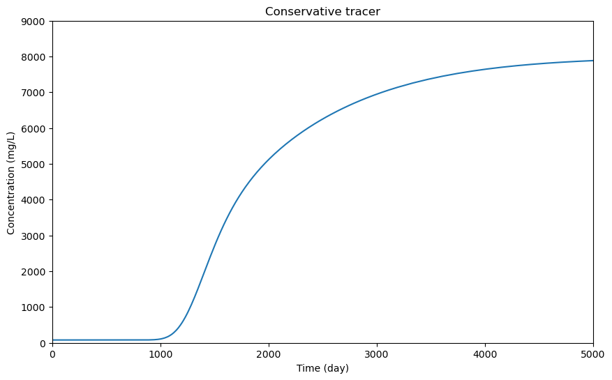
[6]:
import matplotlib.pyplot as plt

# Plot the data using matplotlib
# (The only change from the first example plot is that now we're
# specifying the figure size, in inches)
fig, ax = plt.subplots(figsize=(10, 6))

# The index of the dataframe is the time step, so we'll plot that along the x-axis
ax.plot(df.index, df["Br-"], label="Bromide")

# In the example above, we used separate commands to set the title, x-axis label, y-axis label,
# and x-axis limits. We can also do this in a single command
ax.set(
    title="Conservative tracer",
    xlabel="Time (%s)" % ts.timeunit,
    ylabel="Concentration (%s)" % ts.unit,
    xlim=(0, 5000),
    ylim=(0, 9000),
)

# Show the plot
plt.show()
2. Loading and Plotting SpatialProfile Data
While TimeSeries objects plot time-varying data from a single grid cell, SpatialProfile objects plot spatially varying data at a single snapshot in time. These can include porosity, permeability, mineral volume fractions, reaction rates, and more. Here’s an example where we plot bromide concentrations from a 2D simulation:
[7]:
# Import the SpatialProfile class
from crunchflow.output import SpatialProfile

# Initialize a SpatialProfile object
# Typically, we'll have CrunchFlow output multiple profiles over the course of
# a simulation. Since these are named sequentially ('conc1.out', 'conc2.out', etc),
# we just have to provide the prefix ('conc') and the folder containing the files
conc = SpatialProfile("conc", folder="output_files")

# These output files are from a 2D simulation of a conservative tracer,
# so that should be reflected in the nx, ny, nz and column attributes
print("Dimensions:", conc.nx, conc.ny, conc.nz)
print("Columns:", conc.columns)

# We can also print the "times" attribute, which is a list of each file's output
# number (i.e., the "1", "2", "3" in 'conc1.out', 'conc2.out', 'conc3.out', etc.)
# There is also the "output_times" attribute, which is the time (in simulation time units)
# that each file was output, but that isn't always read in automatically (it depends
# on the version of CrunchFlow/CrunchTope you have)
print("Output numbers:", conc.times)
Dimensions: 100 20 1
Columns: ['Br-']
Output numbers: [1, 2, 3, 4, 5, 6]
[8]:
# To save computation time, the data is not read in immediately. Instead, we can read
# in the data to a numpy array using the `extract` method. Simply provide the name of
# the variable to extract and the time step at which to extract it.
data = conc.extract("Br-", time=1)
print("Minimum concentration (mol/L): %0.5f" % 10 ** data.min())
print("Maximum concentration (mol/L): %0.5f" % 10 ** data.max())
Minimum concentration (mol/L): 0.00100
Maximum concentration (mol/L): 0.00124
[9]:
# Create a plot of Br- concentrations for the first 4 time steps
# Note: the (4, 1) specifies that we want 4 rows and 1 column. `sharex`
# specifies that all subplots should share the same x-axis
fig, axs = plt.subplots(4, 1, figsize=(8, 8), sharex=True)

# Loop over each axis object in the list
# Note that `i` is a counter
for i, ax in enumerate(axs):
    # Extract the data for the current time step
    # (Note that `i` starts at zero, but the time steps start at 1)
    data = conc.extract("Br-", time=i + 1)

    # Plot the data as an image, saving the handle of the image
    # object (`im`) since we will use that later.
    # Note that CrunchFlow outputs logged values, so we need to
    # take 10 to the power of the data to get the actual concentrations.
    # Also, note that we set vmin and vmax (min and max color ranges) to
    # ensure that the colorbar is consistent across all subplots.
    im = ax.imshow(10**data, origin="lower", vmin=0.001, vmax=0.1)

    # Set the ylabel and title for the current subplot
    ax.set(ylabel="Y", title="Time %d" % (i + 1))

# Add x-axis label to the last subplot
axs[-1].set(xlabel="X")

# Add a colorbar to the plot
fig.colorbar(im, ax=axs, label="Concentration (mol/L)", shrink=0.7)

# Show the plot
plt.show()

[10]:
# To understand the concentration patterns in the plot above,
# we can plot permeability and see that the tracer is moving
# around some low-permeability zones
perm = SpatialProfile("permeability", folder="output_files")

# Plot permeability at the first time step
fig, ax = plt.subplots(figsize=(8, 6))

# Extract the permeability data
data = perm.extract("X-Perm", time=1)

# Plot it using a different cmap (colormap) to differentiate it
# from the concentration plots above.
im = ax.imshow(data, origin="lower", cmap="cividis")

# Add a colorbar
fig.colorbar(im, ax=ax, label="log(permeability)", orientation="horizontal", shrink=0.7)

# Add axis labels
ax.set(xlabel="X", ylabel="Y")

plt.show()
